
Sorting is one of the basic operations in data processing and is widely used in programming. Choosing effective sort algorithms is essential for optimizing programs and speeding up the processing of large amounts of information.
I compared three popular sorting algorithms, Merge Sort, Quick Sort, and Heap Sort, to evaluate their efficiency in processing different amounts of data. The study aims to estimate the execution time of each of these algorithms and the number of exchanges made with the same input data.

To do this, several measurements of the execution time of the algorithms were made for different sizes of arrays and various types of data. New data sets were generated three times for each type (integers and real numbers) and the input data size (1000, 10000, and 100000 elements). Each algorithm was run 5 times on the same input data to obtain stable results. Thus, 15 measurements were performed for the same type and size of the input data.
The sorting algorithms were implemented in C, which significantly increases the program’s efficiency in terms of the speed of algorithm execution.
Cocoa and Objective-C were chosen for the development of the graphical interface. C has native compatibility with Objective-C, allowing you to call functions from C within the Objective-C program seamlessly. This provides high sorting performance with minimal costs for interaction between different parts of the program.
Algorithms Overview
Merge Sort is a stable algorithm that uses a divide-and-conquer strategy. Its worst-case time complexity is O(nlogn), making it quite efficient for large amounts of data. MergeSort requires additional space of O(n).
void merge(int arr[], int left, int mid, int right)
{
   int n1 = mid - left + 1;
   int n2 = right - mid;


   int L[n1], R[n2];


   for (int i = 0; i < n1; i++)
       L[i] = arr[left + i];
   for (int j = 0; j < n2; j++)
       R[j] = arr[mid + 1 + j];


   int i = 0, j = 0, k = left;
   while (i < n1 && j < n2)
   {
       if (L[i] <= R[j])
       {
           arr[k] = L[i];
           i++;
       }
       else
       {
           arr[k] = R[j];
           j++;
       }
       k++;
       swapCounter++;
   }


   while (i < n1)
   {
       arr[k] = L[i];
       i++;
       k++;
       swapCounter++;
   }


   while (j < n2)
   {
       arr[k] = R[j];
       j++;
       k++;
       swapCounter++;
   }
}


void mergeSort(int arr[], int left, int right)
{
   swapCounter = 0;
   if (left < right)
   {
       int mid = left + (right - left) / 2;


       mergeSort(arr, left, mid);
       mergeSort(arr, mid + 1, right);


       merge(arr, left, mid, right);
   }
}
Code language: JavaScript (javascript)
Quick Sort is one of the most efficient sorting algorithms. Its average time complexity is O(nlogn), but in the worst case, it can be O(n2), which should be considered when evaluating. QuickSort is generally faster than MergeSort and HeapSort, even though the worst-case time complexity is O(n2). QuickSort sorts the array in place, avoiding the need for additional memory like MergeSort.
int swapCounter = 0;


int partition(int *array, int low, int high)
{
   int pivot = array[high];
   int i = (low - 1);


   for (int j = low; j < high; j++)
   {
       if (array[j] <= pivot)
       {
           i++;
           int temp = array[i];
  array[i] = array[j];
           array[j] = temp;
           swapCounter++;
       }
   }


   int temp = array[i + 1];
   array[i + 1] = array[high];
   array[high] = temp;
   swapCounter++;
   return (i + 1);
}


void quickSortExecute(int *array, int low, int high)
{
   if (low < high)
   {
       int pi = partition(array, low, high);
       quickSortExecute(array, low, pi - 1);
       quickSortExecute(array, pi + 1, high);
   }
}


void quickSort(int *array, int low, int high)
{
   swapCounter = 0;
   quickSortExecute(array, low, high);
}
Code language: PHP (php)
Heap Sort is an algorithm that uses a data structure called a heap. Its time complexity is also O(nlogn), making it consistently efficient even in the worst case. HeapSort also sorts in place but has more overhead due to tree-based operations.
void swap(int *a, int *b)
{
   int temp = *a;
   *a = *b;
   *b = temp;
   swapCounter++;
}


void heapify(int arr[], int n, int i)
{
   int largest = i;
   int left = 2 * i + 1;
   int right = 2 * i + 2;


   if (left < n && arr[left] > arr[largest])
       largest = left;


   if (right < n && arr[right] > arr[largest])
       largest = right;


   if (largest != i)
   {
       swap(&arr[i], &arr[largest]);
       heapify(arr, n, largest);
   }
}


void heapSort(int arr[], int n)
{
   swapCounter = 0;
   for (int i = n / 2 - 1; i >= 0; i--)
   {
       heapify(arr, n, i);
   }
   for (int i = n - 1; i > 0; i--)
   {
       swap(&arr[0], &arr[i]);
       heapify(arr, i, 0);
   }
}
Code language: JavaScript (javascript)
Problem statement
When solving a sorting problem, an important step is correctly choosing the data structure and types to use. For this problem, an array was selected as the data structure. The choice of arrays as the data structure is justified and appropriate for this problem for several reasons. First, arrays provide fast access to elements by index (access time to an element is O(1)), which is essential for most sorting algorithms. For example, algorithms like Quick Sort and Merge Sort often use indexing to exchange or compare elements, making arrays convenient for such operations. In addition, arrays are simple to implement and do not require additional memory costs, unlike complex data structures such as trees or graphs.
Regarding the data type, integers and real numbers were chosen for sorting for several reasons. First, unlike strings, numeric data has a unique order, which makes them ideal for sorting. Comparing numbers is straightforward and efficient, allowing sorting algorithms to work quickly and without the additional time spent processing complex comparisons typical of strings. In the case of string sorting, the comparison involves comparing each character by their ASCII codes or other characteristics, which can be slower than comparing numbers. Moreover, sorting numbers is fundamental to many real-world problems, such as financial data processing, scientific analysis, statistical processing, etc.
Workflow
The algorithm for solving the problem includes several stages: generating input data, measuring the execution time of algorithms, counting operations, and plotting.
- Initialization and selection of parameters:
- Choosing the data type.
- Choosing the set of input data sizes for testing: 1000, 10000, 100000.
- Choosing of three sorting algorithms for comparison: Merge Sort, Quick Sort, and Heap Sort.
- Generating random input data. A random set of numbers is generated using the rand() function for each array size. A random number generator fills the array before starting the time measurement.
For an array of integers, random integers from 0 to 999999 are generated:
 for (int i = 0; i < size; i++) {
           self.arrayInteger[i] = rand() % 1000000;
       }
Code language: HTML, XML (xml)- Random integers from −999.999 to 999.999 are generated for an array of real numbers. When forming the array, there is a 50% probability that the numbers will be negative.
clock_t start = clock();
       mergeSort(array, 0, dataSize - 1);
       clock_t end = clock();
       double time_taken = ((double)end - start) / CLOCKS_PER_SEC;
executionTime = time_taken;Code language: PHP (php)- I use a timer to measure the execution time of each algorithm using the clock() function from the <time.h> library.
- Calculating the average execution time. After collecting the results, the average execution time is calculated for each algorithm, and each array size averageTime = totalTime / 15.
Results
The obtained results of the algorithm execution time (ms *10-4) for integer and real numbers are presented in the table:
Sort | Array Size | |||||
| 1000 | Real vs Integer | 10,000 | Real vs Integer | 100,000 | Real vs Integer | |
| Merge Integer | 3.1166 | -7.5% | 38.7986 | 8.79% | 269.3200 | 6.4% |
| Merge Real | 2.8826 | 42.2086 | 286.5833 | |||
| Heap Integer | 4.0786 | 0.99% | 53.1086 | 5.07% | 365.6106 | 5.41% |
| Heap Real | 4.1193 | 55.8026 | 385.3926 | |||
| Quick Integer | 2.0666 | 7.9% | 26.4866 | 7.1% | 203.3046 | 5.05% |
| Quick Real | 2.2306 | 28.3673 | 213.5746 | |||
Based on these data, we construct graphs for the operation of algorithms with integers and real numbers:

Figure 1 – Running time (ms *10-4) of algorithms for integer numbers
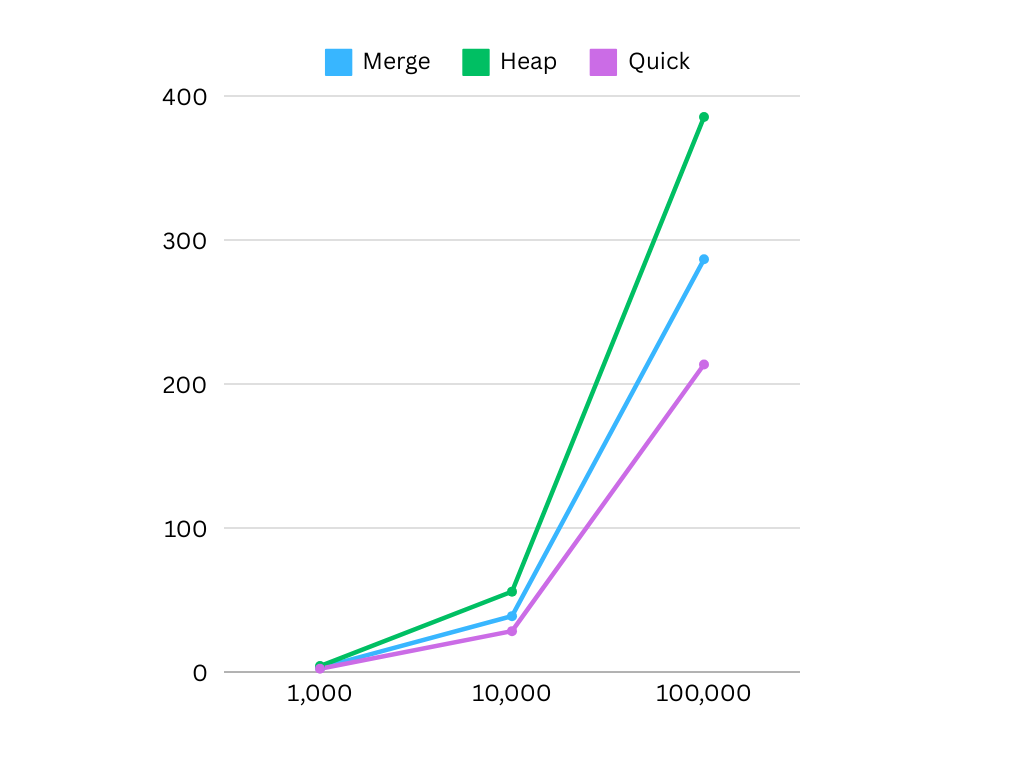
Figure 2 – Running time (ms *10-4) of algorithms for data with real numbers
The number of exchange results for the same array is always the same. We obtained three different values for each separately generated array type and calculated the average. The obtained average results of the number of exchange operations are presented in the table:
Sort | Array Size | ||
| 1000 | 10,000 | 100,000 | |
| Merge Integer | 1,993 | 19,994 | 199,993 |
| Merge Real | 1,993 | 19,994 | 199,993 |
| Heap Integer | 9,044 | 124,267 | 1,575,017 |
| Heap Real | 9,067 | 124,093 | 1,574,953 |
| Quick Integer | 5,800 | 85,827 | 1,075,677 |
| Quick Real | 6,677 | 90,721 | 1,087,087 |
MergeSort avoids swaps. MergeSort primarily uses copy operations instead of swaps. It merges elements into a new array, making fewer direct swaps. MergeSort makes fewer swaps because it merges elements rather than swapping them.
QuickSort and HeapSort require more swaps than MergeSort, with QuickSort being the fastest of the three algorithms and HeapSort being the slowest. QuickSort requires more swaps than MergeSort because QuickSort relies on partitioning by swapping elements. The partitioning step involves swapping elements several times. This increases the total number of swaps. QuickSort is generally faster due to cache efficiency and in-place sorting.
HeapSort performs more comparisons than QuickSort and requires frequent element moves through heap operations. It sorts in place but has poor cache utilization due to the distributed nature of the heap.
Conclusions
- Runtime of sorting algorithms.
Quick Sort was faster than the other two algorithms for all cases.
For Heap Sort, the most extended runtime among the three algorithms is observed for sorting integers and real numbers.
In all three algorithms, the runtime increases with increasing number of elements, which is logical and expected. - Number of exchanges. In all tests for Merge Sort, the number of exchanges remained stable and the same for each input size. This confirms that this algorithm performs a fixed number of exchanges, regardless of their size.
For Heap Sort, the number of exchanges is significantly higher than Merge Sort, which reflects a more complex process of distributing elements in the array through the construction and correction of the heap. In particular, for 100,000 elements, the number of exchanges significantly exceeds the value of Merge Sort.
For Quick Sort, the number of exchanges is also significantly higher than for Merge Sort, particularly for large data sets (100,000 elements), a characteristic feature of this algorithm. - Efficiency of algorithms for different data types. Comparing the results for integers and real numbers shows that in 8 out of 9 cases, the sorting algorithms work better for arrays of integers. On average, integer arrays are sorted 4.3566% faster.
Given these results, all three algorithms work effectively for small data sets, but Quick Sort is the best choice for large amounts of data.