Introduction
Generative Adversarial Networks (GANs) are a hot topic in machine learning for several good reasons. Here are three of the best:
- GANs can provide astonishing results, creating new things (images, texts, sounds, etc.) by imitating samples they have previously been exposed to.
- A GAN offers a new paradigm in machine learning – a generative one – that combines pre-existing techniques to provide both current and brand new ideas and results.
- GANs are a recent (2014) creation of Ian Goodfellow, the former Google, now Apple, researcher (also the co-author of a standard reference in deep learning with Joshua Bengio and Aaron Courville).
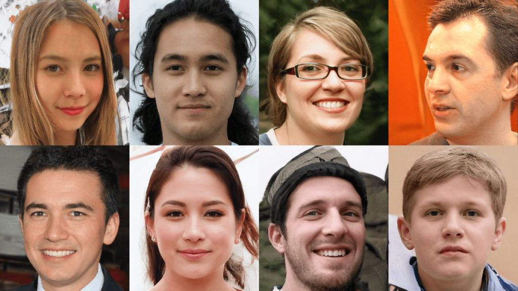
It is likely that readers will already have encountered some of the impressive results GANs are capable of, especially in the realm of image processing. Such networks are able, upon request, to draw a picture of a red flower, a black bird or even a violet cat. Furthermore, that flower, bird, or cat does not exist at all in reality, but is entirely the product of the network’s ‘imagination’.

How is this possible, and can we share in the fun? This article endeavours to address both questions, using functional Python code that can be run on your laptop. You may need to add some packages that are missing from your Python installation, but that’s what Pip is there for…
What is a Generative Adversarial Network?
Neural networks (NNs) were devised as prediction and classification models. They are powerful, non-linear optimizers which can be trained to evolve their inner parameters (neuron weights) to fit the training data. This will enable the NN to predict and classify unknown data of the same kind.
We all know how impressive the data approximations of neural networks, in which ‘data‘ can mean just about anything, can be. However, the features of such algorithms also suggest some of their drawbacks, such as:
- Neural networks need labelled data to be trained properly
- Worse, they need a lot of labelled data
- Worse still, we generally have no idea what the contents of a neuron actually do, except in some special cases
Intrinsically, neural networks are supervised algorithms. Nonetheless, some of their variants work perfectly well as unsupervised algorithms. These can be trained on any kind of data, without requiring the ‘label‘ usually attached to enable the network to differentiate known things from unknown things.
Unsupervised networks have previously been discussed in my articles, using the example of dealing with time series. Any time series may be thought of as a labelled training set if it points to the prediction, while any remaining series provide the input data (see this article for more details).
The GAN paradigm offers another interesting unsupervised setting for neural networks to play in, and is decribed briefly below.
Let us begin with the words the acronym GAN stands for: generative, adversarial, networks. The last is the most obvious – networks: GANs are built up using (usually deep) neural networks. A GAN starts out with an input layer with a certain amount of parallel input neurons (one for each number represented by the input data), some hidden layers and an output layer, connected in a directed graph and trained by a variant of the gradient-descent backpropagation algorithm.
Next, we come to the word generative, which denotes the aim of this class of algorithms. They produce rather than consume data. More specifically, the data these algorithms produce contains new information of the same ‘class’ as the input data used to generate it. The generation process is not spontaneous, but data are generated from other data, via a mechanism that will be described later.
Finally, the word adversarial – the most mysterious term in the acronym – explains how generation occurs, namely through a competition between two adversaries. In the case of a GAN, the adversaries are neural networks.
Therefore, a GAN aims at generating new data via networks deliberately set up in competition with each other in order to achieve this goal. A GAN is always split into two components – two neural (usually deep) networks. The first is known as the discriminator, and it is trained to distinguish a set of data from pure noise. For example, the input data could include a collection of photos of flowers as well as a huge number of other images which have nothing to do with flowers. Each photo may not have an explicit label, but which photos belong to the collection of flowers, and which do not, is known.
The network can then be trained to differentiate flowers from non-flowers or, for that matter, to distinguish photos from pictures created from random pixels. This first ‘discriminator’ component of the GAN is a standard network trained to classify things. The input is an example of the data we want to generate (a collection of photos of flowers if we want to generate flower images), while the output is a yes/no flag.
The other network is the generator: this produces as output the kind of data the discriminator is trained to identify. To achieve this output, the generator uses a random input. Initially this will produce a random output, but the generator is trained to backpropagate the information, whether or not its output is similar to the desired data (e.g., photos of flowers).
To that end, the generator’s predictions are fed into the discriminator. The latter is trained to recognize genuine flowers (in this example), so if the generator can counterfeit a flower sufficiently well to trick the discriminator, then our GAN can produce fake photos of flowers that a well trained observer (the discriminator) will take for the genuine article.
At last, our generation task is accomplished.
One way to think of a GAN is as a room where a forger and an art critic meet: the former offers fake paintings, affirming their authenticity; the latter tries to confirm whether or not they actually are the real deal. If the forger is so good at counterfeiting that the critic mistakes the fakes for the original paintings, then the fakes may be offered at auction in the hope that someone will buy them…
At first glance, GANs may seem to be analogous to reinforcement learning, but the apparent similarity does not stand up to scrutiny. A GAN sets up two networks in competition with each other – the goal is to augment their opposing skills in order to produce fake data that seems genuine. Reinforcement learnng, on the other hand, checks a single agent against an environment and either ‘reinforces’ or ‘punishes’ the agent to correct its behaviour. There’s no competition – just a pattern that needs to be discovered in order to survive.
Instead, GANs may be thought of as a generalisation of the Turing test principle: the discriminator is the tester and the generator the machine willing to pass it, the only difference is that in this case both actors are machines ( see here for more detail on why Turing’s ideas were seminal for machine learning).
A homemade GAN
GANs usually find their most spectacular applications in counterfeiting images, as already discussed. However videos, texts, and even sounds may be generated, although technical issues can complicate the implementation of such ‘time series generators’.
In most tutorials, classic image generation is demonstrated, typically by using the MNIST dataset to teach the GAN how to write letters and digits. However, convolutional networks are required for this process, and the GAN element itself is often neglected in favour of details about setting up the convolutional and ‘deconvolutional’ networks which implement the discriminator and generator. In addition, training is quite a long process when appropriate equipment is lacking (a description of such GANs can be found in another contribution to the Codemotion magazine).
Instead, what follows is an explanation of a simple GAN programmed in Python, using the Keras library (which can be run on any laptop) to teach it how to draw a specific class of curves. I’ve chosen sinusoids, but any other pattern would work equally well.
Below, I’ll demonstrate how to:
- Generate a dataset of sinusoids;
- Set up the discriminator and generator networks;
- Use these to build up the GAN;
- Train the GAN, showing how to combine the training of its components, and;
- Contemplate a somewhat skewed and distorted sinusoid drawn by the program from pure noise.
An artificial dataset
Instead of a collection of images, I’ll produce a description of the curves I am interested in: sinusoids may be mathematically described as the graph of functions
a sin(bx+c)
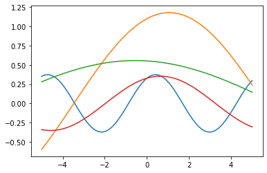
where a, b, c are parameters which determine the height, frequency and phase of the curve. Some examples of such curves are plotted in the following picture, produced via a Python snippet.
import matplotlib.pyplot as plt
import numpy as np
from numpy.random import randint, uniform

X_MIN = -5.0
X_MAX = 5.0
X_COORDS = np.linspace(X_MIN , X_MAX, SAMPLE_LEN)
fig, axis = plt.subplots(1, 1)
for i in range(4):
    axis.plot(X_COORDS, uniform(0.1,2.0)*np.sin(uniform(0.2,2.0)*X_COORDS + uniform(2)))Code language: JavaScript (javascript)
We want our GAN to generate curves with this sort of form. To keep things simple we consider a=1 and let b∈[1/2,2] and c∈[0,π].
First, we define some constants and produce a dataset of such curves. To describe a curve, we do not use the symbolic form by means of the sine function, but rather choose some points in the curve, sampled over the same x values, and represent the curve y = f(x) by the vector (y1,…,yN) where yi = f(xi) for the fixed xs.
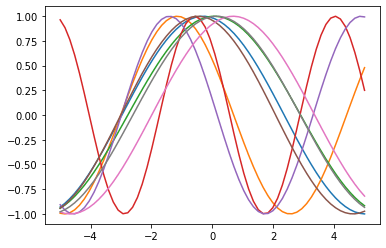
The y values are generated by using the previous formula for random values of b and c within the prescribed intervals. Having definined the training set, some of these curves can be plotted.
import numpy as np
from numpy.random import uniform

import matplotlib.pyplot as plt

SAMPLE_LEN = 64       # number N of points where a curve is sampled
SAMPLE_SIZE = 32768   # number of curves in the training set
X_MIN = -5.0          # least ordinate where to sample
X_MAX = 5.0           # last ordinate where to sample

# The set of coordinates over which curves are sampled
X_COORDS = np.linspace(X_MIN , X_MAX, SAMPLE_LEN)

# The training set
SAMPLE = np.zeros((SAMPLE_SIZE, SAMPLE_LEN))
for i in range(0, SAMPLE_SIZE):
    b = uniform(0.5, 2.0)
    c = uniform(np.math.pi)
    SAMPLE[i] = np.array([np.sin(b*x + c) for x in X_COORDS])

# We plot the first 8 curves
fig, axis = plt.subplots(1, 1)
for i in range(8):
    axis.plot(X_COORDS, SAMPLE[i])Code language: PHP (php)
Our GAN in small pieces
Next we define our discriminator, namely the neural network used to distinguish a sinusoidal curve from any other set of sampled points. The discriminator consequently accepts an input vector (y1, …, yN) and returns 1 if it corresponds to a sinusoidal curve, otherwise 0.
The Keras library is then used to create a Sequence object in which to stack the different layers of the network. This discriminator is arranged as a simple shallow multilayer perceptron, with three layers: the input layer with N neurons, N being the size of the input vectors, a second layer with the same number of hidden neurons, and a third with just one neuron, the output layer.
The output of the input and hidden layers is filtered by a ‘relu’ function (which cuts negative values of its argument x) and by a ‘dropout’ (which randomly sets input units to 0 at a prescribed frequency during each step of training, to prevent overfitting).
The output neuron is activated via a sigmoid function which smoothly extends from 0 to 1, the two possible answers.
from keras.models import Sequential
from keras.layers import Dense, Dropout, LeakyReLU

DROPOUT = Dropout(0.4)        # Empirical hyperparameter
discriminator = Sequential()
discriminator.add(Dense(SAMPLE_LEN, activation="relu"))
discriminator.add(DROPOUT)
discriminator.add(Dense(SAMPLE_LEN, activation="relu"))
discriminator.add(DROPOUT)
discriminator.add(Dense(1, activation = "sigmoid"))
discriminator.compile(optimizer = "adam", loss = "binary_crossentropy", metrics = ["accuracy"])Code language: PHP (php)
Next we come to the generator network. This is in a sense a mirror of the discriminator; we still have three layers, in which the input layer accepts a noisy input of the same size as the output (a vector with N elements), and applies a ‘leaky relu’ function (which cuts negative values of its argument x to a small multiple of x itself). However, this network does not perform dropout, and outputs the result via a hyperbolic tangent function. Since classification is not our goal, we use mean square error as the loss function instead of binary cross entropy when training the network and using it to make predictions.
LEAKY_RELU = LeakyReLU(0.2)   # Empirical hyperparameter
generator = Sequential()
generator.add(Dense(SAMPLE_LEN))
generator.add(LEAKY_RELU)
generator.add(Dense(512))
generator.add(LEAKY_RELU)
generator.add(Dense(SAMPLE_LEN, activation = "tanh"))
generator.compile(optimizer = "adam", loss = "mse", metrics = ["accuracy"])Code language: PHP (php)
Next, we plug the output of the generator into the discriminator as input, so that the whole GAN network is ready to be trained.
gan = Sequential()
gan.add(generator)
gan.add(discriminator)
gan.compile(optimizer = "adam", loss = "binary_crossentropy", metrics = ["accuracy"])Code language: JavaScript (javascript)
How is a GAN trained?
The GAN is now ready to be trained. Instead of immediately launching the fit Keras method on the gan object we just instantiated, let’s pause and reflect on the concept of GAN to understand how to train it properly.
As has already been stated, the discriminator needs to learn how to distinguish between a sinusoid and another curve. This can be done by simply training it on our SAMPLES dataset and a noisy dataset, labelling elements in the former sinusoids, and in the latter non-sinusoids.
However, the aim of the discriminator is not merely to learn our dataset but to intercept the fakes produced by the generator. With this in mind, the discriminator is trained as follows:
- For each epoch, a batch training is performed on both the discriminator and the generator.
- This batch training starts by asking the generator to generate a batch of curves.
- The output of this is coupled to a batch of sinusoids from our
SAMPLEdataset, and a dataset with labels 1 (=genuine sinusoid) and 0 (=sinusoid produced by the generator) is provided to batch train the discriminator, which is thereby trained to recognise the generated sinusoid among the genuine examples. - The generator is batch trained on random data: this training backpropagates along the whole GAN network, but weights in the discriminator are left untouched.
The result is that the discriminator is not trained to recognize sinusoids, but to distinguish between sinusoids from our datasets and sinusoids produced by the generator. Meanwhile, the generator is trained to produce sinusoids from random data in order to deceive the discriminator.
When the success rate of this deception is high (from the point of view of the discriminator), the GAN is able to generate fake sinusoids. Because we want the code to run without starving our laptops (which can be assumed in the absence of GPUs etc.) relatively small parameters are used to produce our dataset and train the GAN. Therefore we cannot expect the network to draw a smooth sinusoid; instead we expect a rather wobbly line that nonetheless displays a sinusoidal pattern.
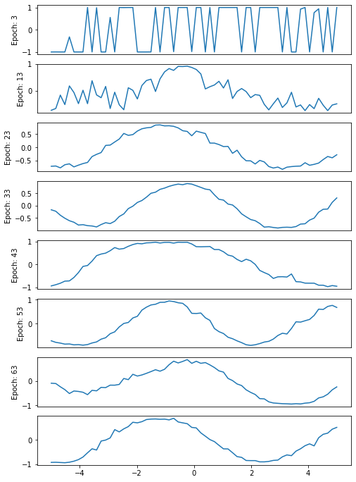
To demonstrate how the GAN starts by drawing randomly, then gradually improves its skill at drawing a sinusoid during its ‘apprenticeship’, I have plotted some of the GAN outputs created during its training (10 epochs are plotted, since we are using just 64 epochs in total).
EPOCHS = 64

NOISE = uniform(X_MIN, X_MAX, size = (SAMPLE_SIZE, SAMPLE_LEN))
ONES = np.ones((SAMPLE_SIZE))
ZEROS = np.zeros((SAMPLE_SIZE))
print("epoch | dis. loss | dis. acc | gen. loss | gen. acc")
print("------+-----------+----------+-----------+----------")

fig = plt.figure(figsize = (8, 12))
ax_index = 1
for e in range(EPOCHS):
    for k in range(SAMPLE_SIZE//BATCH):
        # Addestra il discriminatore a riconoscere le sinusoidi vere da quelle prodotte dal generatore
        n = randint(0, SAMPLE_SIZE, size = BATCH)
        # Ora prepara un batch di training record per il discriminatore
        p = generator.predict(NOISE[n])
        x = np.concatenate((SAMPLE[n], p))
        y = np.concatenate((ONES[n], ZEROS[n]))
        d_result = discriminator.train_on_batch(x, y)
        discriminator.trainable = False
        g_result = gan.train_on_batch(NOISE[n], ONES[n])
        discriminator.trainable = True
    print(f" {e:04n} |  {d_result[0]:.5f}  |  {d_result[1]:.5f} |  {g_result[0]:.5f}  |  {d_result[1]:.5f}")
    # At 3, 13, 23, ... plots the last generator prediction
    if e % 10 == 3:
        ax = fig.add_subplot(8, 1, ax_index)
        plt.plot(X_COORDS, p[-1])
        ax.xaxis.set_visible(False)
        plt.ylabel(f"Epoch: {e}")
        ax_index += 1

# Plots a curve generated by the GAN
y = generator.predict(uniform(X_MIN, X_MAX, size = (1, SAMPLE_LEN)))[0]
ax = fig.add_subplot(8, 1, ax_index)
plt.plot(X_COORDS, y)Code language: PHP (php)
The output is:
epoch | dis. loss | dis. acc | gen. loss | gen. acc
------+-----------+----------+-----------+----------
 0000 |  0.10589  |  0.96484 |  7.93257  |  0.96484
 0001 |  0.03285  |  1.00000 |  8.62279  |  1.00000
 0002 |  0.01879  |  1.00000 |  9.54678  |  1.00000
 0003 |  0.01875  |  1.00000 |  11.18307  |  1.00000
 0004 |  0.00816  |  1.00000 |  13.98673  |  1.00000
 0005 |  0.01707  |  0.99609 |  16.46034  |  0.99609
 0006 |  0.00579  |  1.00000 |  13.86913  |  1.00000
 0007 |  0.00189  |  1.00000 |  17.36512  |  1.00000
 0008 |  0.00688  |  1.00000 |  17.61729  |  1.00000
 0009 |  0.00306  |  1.00000 |  18.18118  |  1.00000
 0010 |  0.00045  |  1.00000 |  24.42766  |  1.00000
 0011 |  0.00137  |  1.00000 |  18.18817  |  1.00000
 0012 |  0.06852  |  0.98438 |  7.04744  |  0.98438
 0013 |  0.20359  |  0.91797 |  4.13820  |  0.91797
 0014 |  0.17984  |  0.93750 |  3.62651  |  0.93750
 0015 |  0.18223  |  0.91797 |  3.20522  |  0.91797
 0016 |  0.20050  |  0.91797 |  2.61011  |  0.91797
 0017 |  0.24295  |  0.90625 |  2.62364  |  0.90625
 0018 |  0.34922  |  0.83203 |  1.88428  |  0.83203
 0019 |  0.25503  |  0.88281 |  2.24889  |  0.88281
 0020 |  0.28527  |  0.88281 |  1.84421  |  0.88281
 0021 |  0.27210  |  0.88672 |  1.92973  |  0.88672
 0022 |  0.30241  |  0.88672 |  2.13511  |  0.88672
 0023 |  0.33156  |  0.82422 |  2.02396  |  0.82422
 0024 |  0.26693  |  0.86328 |  2.46276  |  0.86328
 0025 |  0.39710  |  0.82422 |  1.64815  |  0.82422
 0026 |  0.34780  |  0.83984 |  2.34444  |  0.83984
 0027 |  0.26145  |  0.90625 |  2.20919  |  0.90625
 0028 |  0.28858  |  0.86328 |  2.15237  |  0.86328
 0029 |  0.34291  |  0.83984 |  2.15610  |  0.83984
 0030 |  0.31965  |  0.86719 |  2.10919  |  0.86719
 0031 |  0.27913  |  0.89844 |  1.92525  |  0.89844
 0032 |  0.31357  |  0.87500 |  2.10098  |  0.87500
 0033 |  0.38449  |  0.83984 |  2.03964  |  0.83984
 0034 |  0.34802  |  0.81641 |  1.73214  |  0.81641
 0035 |  0.28982  |  0.87500 |  1.74905  |  0.87500
 0036 |  0.33509  |  0.85156 |  1.83760  |  0.85156
 0037 |  0.29839  |  0.86719 |  1.90305  |  0.86719
 0038 |  0.34962  |  0.83594 |  1.86196  |  0.83594
 0039 |  0.32271  |  0.84766 |  2.21418  |  0.84766
 0040 |  0.31684  |  0.84766 |  2.22909  |  0.84766
 0041 |  0.37983  |  0.83984 |  1.79734  |  0.83984
 0042 |  0.31909  |  0.83984 |  2.10337  |  0.83984
 0043 |  0.30426  |  0.86719 |  1.98194  |  0.86719
 0044 |  0.30465  |  0.86328 |  2.31558  |  0.86328
 0045 |  0.35478  |  0.84766 |  2.40368  |  0.84766
 0046 |  0.30423  |  0.86328 |  1.93115  |  0.86328
 0047 |  0.30887  |  0.83984 |  2.17885  |  0.83984
 0048 |  0.35123  |  0.86719 |  2.00351  |  0.86719
 0049 |  0.24366  |  0.90234 |  2.21016  |  0.90234
 0050 |  0.33797  |  0.84375 |  1.99375  |  0.84375
 0051 |  0.35846  |  0.84375 |  2.17887  |  0.84375
 0052 |  0.35476  |  0.83203 |  2.15312  |  0.83203
 0053 |  0.28164  |  0.87109 |  2.60571  |  0.87109
 0054 |  0.25782  |  0.89844 |  1.87386  |  0.89844
 0055 |  0.28027  |  0.87500 |  2.30517  |  0.87500
 0056 |  0.31118  |  0.84375 |  2.00939  |  0.84375
 0057 |  0.32034  |  0.85547 |  2.22501  |  0.85547
 0058 |  0.34665  |  0.84375 |  2.11842  |  0.84375
 0059 |  0.32069  |  0.85547 |  1.79891  |  0.85547
 0060 |  0.32578  |  0.87500 |  1.85051  |  0.87500
 0061 |  0.32067  |  0.87109 |  1.70326  |  0.87109
 0062 |  0.31929  |  0.85938 |  1.99901  |  0.85938
 0063 |  0.38814  |  0.83984 |  1.55212  |  0.83984
[<matplotlib.lines.Line2D at 0x1b5c3054c48>]Code language: HTML, XML (xml)
Notice that the first picture, after three epochs, is more or less random, while the subsequent images move towards a smoother curve (even if our 64 epochs are not enough for a really good curve!) and, more importantly, towards a curve that displays a sinusoidal trend.
What can also be observed is the progress of loss and accuracy for both the discriminator and the whole generative network during training. On examining this log we can see that the lower the loss value of the GAN, the better the curve approximates a sinusoid. Finally, on examining the values for the discriminator, it is clear that some adjustments in the hyper-parameters (or even in the architecture of the networks) are in order.
Conclusions
The example we have played with here may not seem especially impressive, but it really should. In the course of this article, two shallow networks have been assembled which (dropout and leaky relu aside) could have been programmed in the late 1980s. However, setting these networks up against each other in competition has produced a generating network that ‘draws’ curves resembling the one fed to it.
Beyond that, the network understands which models to imitate from just a small sample description, and running the programs on your computer has probably taken a few minutes at most.
By combining more sophisticated networks along the same lines, a GAN able to generate digits, letters, or more complex figures can be created. Some modifications in the training techniques and in the representation of data would allow the GAN to generate speeches, videos, and in the near future, anything of which there are plenty of examples on the Web, which is to say, almost everything!
Recommended Article: Top Trending Python Frameworks


